gBay Wiki

A Bayesian Network is a directed, acyclic graph with an underlying joint probability distribution. It therefore consists of three parts:

• A set of nodes representing variables, each with a set of mutually exclusive (discrete or continuous) states.
• A set of links representing the (directed) causal relationships or dependencies between these nodes.
• A set of probabilities specifying the belief that a node X will be in a particular state for each combination of its parent nodes’ Pa(X) states (conditional probability tables - CPTs).

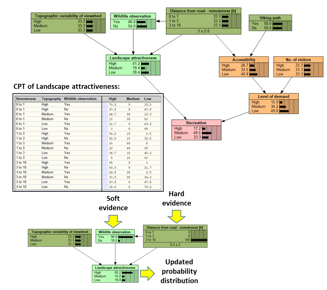
Once the BN is compiled, we running by adding evidence to one or more nodes, which is propagated through the network and the joint probability distribution is updated. This calculation is called inference, and it is performed by applying Bayes’ theorem:

$ P(X) = ∑Pa(X)P(X|Pa(X)) * P(Pa(X))$

Evidence can be data (e.g. when we know the type of land cover in a pixel) or scenarios (e.g. when we explore what happens in the system when we increase the harvesting rate). When we know the state of a node with 100% certainty, this is called hard evidence (the land cover is a forest), while soft evidence contains some uncertainty and is in the form of a probability distribution (the land cover is a forest with 70% probability and a grassland with 30% probability).

Example of a Bayesian Network that describes the ecosystem service of recreation. The CPT of node “Landscape attractiveness” is shown, as well as how the probability distribution of this node is updated when we add evidence to its parent nodes. For more details on this network, Example x.

Before the construction of the BN begins, it is important to clarify the problem and objectives, as well as the modelling context:

• What is the main question to be addressed with the model? What are the “target nodes” – the main variables of interest, e.g. the focal ecosystem services?
• What are the key drivers that affect the focal ecosystems?
• How will the model be used? BNs can be used to improve system understanding, for scenario or trade-off analysis, to support and inform management, to understand uncertainties, or for several of these purposes. The complexity of the model and the methods used to construct it should be adapted to its aim and target audience. For example, a simpler BN is more suited to communicate with stakeholders, while a more complex model may help integrate various data and models, to produce more accurate ES maps. Furthermore, if a BN is aimed at communicating with stakeholders or managers, these should be involved in the development of the network and agree with its purpose.
• What is the appropriate spatial scale and extent to address the question?
• Should the model be dynamic, i.e. take into account multiple time steps? If so, what is the appropriate temporal resolution?

A variety of Bayesian Network software packages is available, such as Hugin, AgenaRisk, Genie, OpenBUGS, and various R packages. In this manual, we demonstrate how to create a BN in Netica, the BN software most commonly used in ecosystem service modelling.

A free test version of Netica (with a limit of 15 nodes per network) can be downloaded at http://www.norsys.com/, and an extensive web help is available at: https://www.norsys.com/WebHelp/NETICA.htm#NETICA/X_Glossary_AE.htm

However, many functionalities are also available in other software packages. For an overview, see review by Pérez-Miñana (2016).

Once the purpose and context of the BN are defined, we select the variables that should be represented as nodes in the network in order to address the question. The BN can include the following sets of variables:

• Focal ecosystem services as target nodes
• Ecosystem properties (structure and processes) that influence the provision of these services
• Controlling factors that affect the relevant ecosystem properties (drivers, pressures)
• Variables describing the demand for the ecosystem service
• Management interventions and scenarios
• Proxies and indicators for variables that cannot be directly assessed, including remote sensing variables

The relevant variables in the system can be defined by experts, from literature, or through stakeholder workshops.

A good way to find a set of relevant influence factors is a workshop with experts or stakeholders. Before the workshop, a list of relevant factors can be compiled based on literature or expert interviews. At the workshop, the participants individually rank the importance of the individual factors. Then, the ranking is discussed to find a consensus about a set of most relevant influence factors (Celio et al. 2014). For more details on setting up a BN with experts or stakeholders, see Cain (2001), Celio et al. (2014), and Salliou et al. (2017).

To create a node in Netica, click on the icon and then place the new node somewhere on the canvas. Double click on the node to open a window with the node properties, where you can change the node name and define it as discrete or continuous.

In the next step, the relationships between the nodes are included as directed links in the network. The links represent causal relationships, not to be mistaken with the flow of information. For example, an EO product such as a land cover classification is an input node to the network, as it provides information about the actual land cover. However, in terms of causality, the classification depends on the actual state, not vice versa, so the link should be directed from the land cover to the classification. Defining links based on causality maintains the logical structure of the network. However, it is not always easy to define causality, and sometimes a pragmatic approach is necessary, where links are defined in a way that facilitates the construction of CPTs.

During this step, we follow the following guidelines:

• Nodes with no parents should represent the state of the ecosystem, driving factors, or management interventions.
• Nodes with no children should be the ES of interest or additional impacts (these only if their inclusion is relevant to the modelled problem).
• If possible, there should not be more than three parents for each child node (the size of a CPT grows exponentially with the number of parents).
• Feedback loops are not allowed in BNs. In case of a feedback effect, consider which direction of impact is more relevant for the modelling purpose and within the temporal and spatial scale of interest. The alternative is to use a dynamic BN, consisting of several BNs at different time steps (see section on dynamic BNs).

The resulting network should be reviewed by other experts, and (if aimed for communication and management) by the relevant stakeholders. During the process, it is often necessary to return to the previous step and define new nodes or redefine existing nodes.

One approach to define the causal links between nodes is using an influence matrix, where experts (or stakeholders) are presented with a matrix based on the list of nodes that they previously agreed on. Then, they are asked to assess the influence of each node on every other node in the network (Celio et al. 2014). This can be done in a workshop or via an (online) questionnaire. The influence matrix can be translated into causal links in the network, which should then be discussed with the experts. As a first step to construct a network, it is necessary, to construct the casualties of all driving factors. Because there is no natural scale for judging direct impact strength, the scale has to be determined, e.g. a 5-point-scale. A problem that might appear is the high amount of impacts. To deal with this phenomenon, the calculation of standard statistics (mean, median, variance) are helpful to show the degree of heterogeneity and to aggregate the experts impact estimations. Based on this a preliminary network can be constructed to be discussed with the experts.

To create a link between two nodes in Netica, click on the arrow icon in the toolbar. Then click on the parent node and drag the arrow to its child node.

For every node in the network, we define whether they should be described as discrete (states are categories, such as land cover) or continuous (e.g. biomass) variables. For discrete variables, a finite set of mutually exclusive states should be defined. The number of states exponentially increases the complexity of the CPTs, and should therefore be kept to a minimum that still represents the states relevant for the system. Continuous variables need to be discretized into intervals, where the number of intervals should be as low as possible, while accounting for any important thresholds and maintaining the shape of the probability distribution.

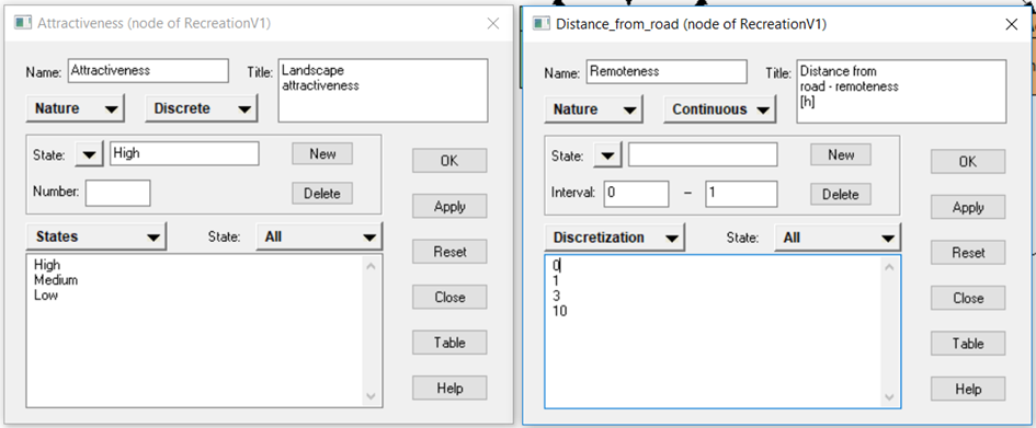
To modify the states of a node in Netica, double click on the node to open the node properties window. Click on “Description” and select “States”. Then, simply enter the names of the states in the box below. For continuous nodes, the states are defined through discretization intervals. Select “Discretization” and enter the threshold values between the states.

Defining states for discrete and continuous nodes in Netica.

The links between nodes in a BN are represented by conditional probability tables, where a probability distribution of a child node is defined for every combination of states of its parent nodes. Depending on the availability of data or models, various methods can be used to populate CPTs, from expert elicitation to “learning” from data. During this process, we may find it necessary to return to previous steps and redefine the nodes, their states, or the links between them.

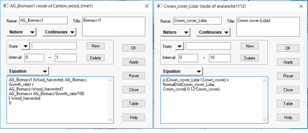
In Netica, the CPTs can be filled either manually (right click on the node → Table) or through equations. To use an equation, open the node properties, select Equation, and enter the equation in the box. Then, click on to calculate the CPT based on the equation.

Examples of a deterministic (left) and probabilistic (right) equation in Netica.

When data is lacking, the CPTs can be filled manually by experts or by stakeholders. Usually, this means that the experts should specify the probability of each state of the child node given each combination of parent nodes. When a node has many parents with several states, many rows of CPTs need to be filled, which can lead to fatigue and boredom, and it is difficult to ensure consistent distributions (Das 2004). This is why it is important to limit the number of parents, and the number of node states.

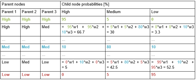
When node states are binary or ordered, this problem can be reduced by using various interpolation methods (Cain 2001, Das 2004). For example, if a child node C has three states (“low”, “medium”, “high”), and three parents Pa with the same three states, we can elicit three probability distributions of C: where all three parents are in state “high”, all in state “medium”, and all in state “low”. In addition, we need the relative weights of each parents (w1, w2, w3, which should sum up to one). Then, all the other rows of the CPT can be calculated by interpolation.

Example of interpolation in a CPT, where the weights of the parents are w1 = 0.17, w2 = 0.5, w3 = 0.33. Elicited probabilities are shown in bold, while all other probabilities in the table are calculated using interpolation, as shown below.

Distributions of continuous variables can also be elicited from experts. One useful approach is the four-point estimation method (Speirs-Bridge et al. 2010), where we ask experts for the expected value of the node for a specific combination of parents, the expected upper and lower bounds of possible values, and their confidence in their estimate. Using this information, we can estimate a probability distribution (e.g. a normal or triangular distribution). An example of this approach is available in the avalanche protection case study.

In some cases, experts find it easier to deal with categories rather than continuous variables, and it may be useful to translate continuous nodes to discrete classes using fuzzy logic.

When using expert elicitation, more than one expert should be involved whenever possible. Then, we can evaluate the differences between the experts, and test the sensitivity of the network to these differences. This may be particularly interesting when developing a network with different stakeholder groups. For a final network, the CPTs are usually combined by averaging the values from different experts.

Some stakeholders may find it difficult to estimate probabilities. In this case, surveys should be designed in a way that is understandable and easy to fill out. In order to understand farmers’ decisions in the Sierra Nevada, a choice experiment was used.

To map ecosystem services, proxies of ecosystem structure are often derived from remote sensing (e.g. land cover classifications or LiDAR-based measurements of vegetation cover). However, these remote sensing products often include some uncertainty due to measurement errors or misclassifications. To make these uncertainties explicit, we can create separate nodes representing the observed value and the actual state of the variable. The observation is caused by the actual state, not vice-versa, and defining the structure of the network based on this causality helps to define conditional probabilities (see avalanche protection case study).

Often, some parts of the network have already been extensively researched and empirical or process-based models are available in literature. In this case, the model can be incorporated in the BN in the form of probabilistic equations. This usually means that the probability distribution of the child node is a normal distribution, where the mean is a function of its parents, and the standard deviation is derived from the reported uncertainty in the model. Other types of distributions can also be used.

For an example of how an empirical model can be incorporated in a BN, see the avalanche protection case study.

Where sufficient data is available, CPTs can be “learned” directly from data within a BN software. Learning a CPT requires a dataset of cases with information on the child node and its parents. Various algorithms (e.g. Expectation Maximisation or gradient descent) can be used to find the maximum likelihood BN, which is the network that is most likely given the data. This approach can also be used to translate process-based simulation models into the BN. We run the simulation over the range of input values, and use the results as cases for learning the BN. Parameters that are not included in the network should also be varied in the simulation, in order to capture the uncertainty in the model.

To “learn” from data in Netica, create a text file where the column names match the names of the nodes in the network, and rows represent cases (i.e. observations, plots, measurements). Go to Cases → Learn → Incorp Case File (to derive CPTs by simply counting the cases) or Learn Using EM (to use the expectation maximisation algorithm, e.g. in case of missing data). To use learning only for the CPT of one node, select the node before performing the learning.

Learning from simulations was used to populate one of the nodes in the avalanche protection network, while in-situ data were used to quantify some nodes in the BN of ecosystem services in the Wadden Sea.

Once all the CPTs in the BN are filled, the network can be compiled. Then, it can be tested by entering “evidence” (modifying the probability of a node, e.g. setting the probability of a specific state to 100%). The evidence is propagated through the network by inference, and we can observe the resulting probabilities in other nodes. The BN and its behaviour under different scenarios should be presented to experts and stakeholders, and evaluated by them. Afterwards, their feedback is used to adjust the structure of the network, the states of the variables, or to update the CPTs.

Sensitivity analysis is a useful tool that determines the influence of individual variables on the outputs, which can help us decide where more data is necessary. When new data becomes available, it can be used to update the conditional probability distributions in an iterative process.

In Bayesian Network modelling, sensitivity analysis is often used to evaluate the influence of variables in the modelled system on the posterior probability distribution of a node of interest (Uusitalo 2007, Marcot 2012). Sensitivity to findings can be measured by the reduction in uncertainty (e.g. entropy or variance) in the target node due to a finding on another node. Entropy reduction is expressed by the measure of mutual information (Kjaerulff and Madsen 2013):

$ I(X,Y) = H(X) - H(X|Y) = H(Y) - H(X|Y)= ∑_Y P(Y)∑_X P(Y)(P(X,Y))/(P(X)P(Y)) $

where H(X) is the entropy of X and H(X|Y) is the entropy of X after a new finding on Y.

The analysis of sensitivity to findings gives us an indication of which variables in the system have the highest influence on the outcome of the model.

To perform sensitivity analysis in Netica, select the node whose sensitivity you want to measure. Then, go to Network → Sensitivity to findings, and you will get a table showing the sensitivity metrics (mutual information, relative mutual information, variance of beliefs, and, for continuous nodes, variance reduction). Sensitivity analysis can be used to map the flow of information in a Bayesian Network and analyse uncertainties.

When co-constructing a BN with experts or stakeholders, it is important that they are presented with the results of the process, and can validate them. In a workshop setting, the participants can input scenarios in the network, see the results, and evaluate whether these agree with their understanding of the system (Celio et al. 2014).